Get acquainted with one of the simplest non-parametric methods used for classification and regression. This method has been used in pattern recognition since the beginning of the 1970s.
Author: Goran Sukovic, PhD in Mathematics, Faculty of Natural Sciences and Mathematics, University
The previous post gives an overview of supervised learning from examples. This article describes one of the simplest non-parametric methods used for classification and regression. K-NN is a non-parametric method and has been used in pattern recognition from the beginning of the 1970s. The input or training examples are vectors in a multidimensional feature space. The output depends on whether K-NN is used for classification or regression:
– For the K-NN classification, the output is a class membership. An input object is assigned to the class most common among its K nearest neighbors. The algorithm uses a majority vote of its neighbors, where K is a small positive integer. If we use 1-NN (i.e., K = 1), then the input is assigned to the class of that single nearest neighbor.
– For the K-NN regression, the output is the average or weighted average of K’s nearest neighbors.
If the function is approximated locally and all the computations are deferred until evaluation, we talk about instance-based learning. K-NN is an instance-based learning method since only the K nearest neighbors are used to calculate the output. The method can be improved by assigning a weight to the contributions of the neighbors, so the nearer neighbors’ contribution is, on average, higher than the contribution of the more distant neighbors. The primary disadvantage of K-NN is sensitivity to the local structure of the data.
The algorithm for classification is very simple; store all available input vectors along with corresponding classes and classify new input cases based on a similarity measure. Similarity measure is represented by distance functions. An input vector is classified by a majority vote of its neighbors. So, the input vector is assigned to the class most common among its K nearest neighbors, measured by a distance function. If K = 1, then the case is simply assigned to the class of its nearest neighbor.
Suppose we have two d-dimensional real vectors (x1, x2, …, xd) and (y1, y2, …, yd). Some distance measures are represented in the following table:
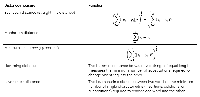
It should be noted that the first three distance measures are only valid for continuous variables. Also, Euclidean distance and Manhattan distance are special cases of the Minkowski distance. In the case of categorical variables, the Hamming distance, Levenshtein distance, or some other suitable distance measure must be used. If the mixture of numerical and categorical variables is presented in the dataset, we have to standardize numerical variables, usually to segment [0, 1] or [-1,1].
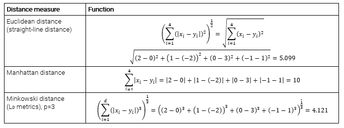
Example 1:
Suppose we have two vectors in R4: x=(2, 1, 0, -1) and y=(0, -2, 3, 1). Then we have:
Example 2 (adapted from Wikipedia):
Hamming distance between strings “karolin” and “kerstin” is 3.
Hamming distance between binary strings “1011101” and “1001001” is 2.
Levenshtein distance between strings “karolin” and “kerstin” is 3, as a Hamming distance.
Levenshtein distance “kitten” and “sitting” is 3. There are 3 edits change: kitten → sitten (substitution of “s” for “k”), sitten → sittin (substitution of “i” for “e”), and sittin → sitting (insertion of “g” at the end). There is no way to transform string “kitten” to “sitting” with less than three edits.
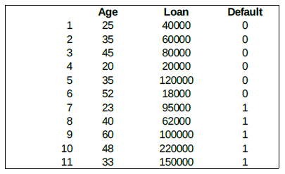
Example 3 (adapted from https://www.saedsayad.com/k_nearest_neighbors.htm):
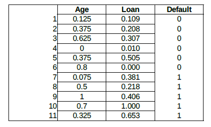
Consider the following data concerning credit default. We have eleven two-dimensional input vectors with two numerical features (predictors), Age and Loan. Default is the target with values 0 (no default) or 1 (default). The training set is:
Our new unknown input vector is (Age=48, Loan=142,000). We can now classify an unknown case using Euclidean distance.
The following table shows the distance from unknown input to all examples of the training sets:
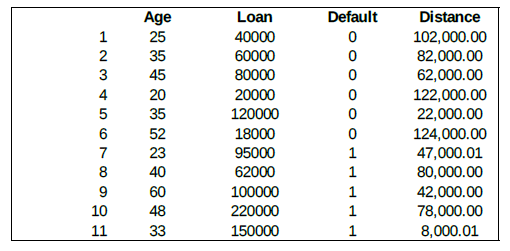
If K=1, then the nearest neighbor is the example 11 (the last one in the training set), so we set Default=1 for the new input vector.
With K=3, the nearest neighbors are examples 11, 5, and 9. Two of them are Default=1, and one is Default=0. The prediction for the unknown input is again Default=0.
You can play with the interactive K-NN algorithm on https://www.saedsayad.com/flash/KNN_flash.html.
In our example, one variable is based on the value of a loan in euros, and the other is based on age in years. The predictor loan will have a much stronger influence than the age on the distance calculated. One solution is to standardize the training set. There are many methods of how to standardize the training set. One of the methods is shown below, where we use the following formula (x-xmin)/(xmax-xmin) to transform all values into a segment [0, 1].
Using the standardized distance on the same training set, the unknown input returned a different neighbor, which is not a good sign of robustness.
One commonly used distance metric for continuous variables is the Euclidean distance or L2 metric. In the case of text classification or other discrete classification tasks, another metric can be used, such as Hamming distance or Levenshtein distance. Even statistical correlation coefficients such as Pearson and Spearman can be used as a metric (for example, in the context of gene expression microarray data). Furthermore, we can use other specialized algorithms, such as Large Margin Nearest Neighbor or Neighborhood components analysis, to learn the distance metric and improve K-NN classification accuracy.
If the class distribution is skewed, the basic “majority voting” classification has an issue with examples of a more frequent class. Due to their large number, these examples tend to be common among the K nearest neighbors and dominate the prediction of the new example. One way to overcome this problem is to weight the classification, taking into account the inverse distance from the test point to each of its K nearest neighbors.
The best choice of K depends upon the data and can be selected by various heuristic techniques. In binary classification problems, it is helpful to choose K to be an odd number as this avoids tied votes. In the case of classification and regression, we can choose the right K for our data by trying several Ks and picking the one that works best.
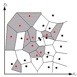
For K=1, the K-NN rule leads to the partition of the space into cells (Voronoi cells), enclosing the training points labeled as belonging to the same class, as shown in the picture below.
For K-NN regression, we can calculate the mean value of the K nearest training examples rather than calculate their most common value.
We gave a short introduction to K-NN. The K-nearest neighbors (K-NN) algorithm belongs to supervised machine learning algorithms and can be used for both classification and regression tasks.
Thanks for reading this article. If you like it, please recommend, and share it.