We give a short introduction to the logistic regression model. Logistic regression is simply an extension of the linear regression model. We introduce a few new statistical concepts, but they are relatively simple and within reach of anyone who can use linear models. Logistic regression provides the foundation for more sophisticated machine learning techniques.
Author: Goran Sukovic, PhD in Mathematics, Faculty of Natural Sciences and Mathematics, University
Many algorithms and techniques in machine learning are borrowed from statistics. To describe properties of population growth in ecology, statisticians developed the logistic function, also called the sigmoid function, given by
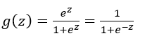
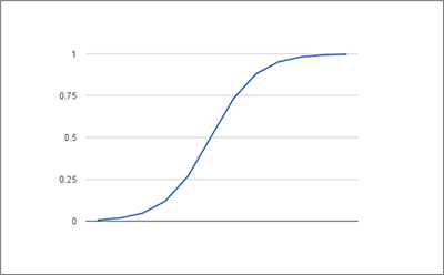
The graph of the sigmoid function is an S-shaped curve that can take any real-valued number and map it to a value between 0 and 1, as it’s shown in Figure 1 (input values are taken from segment [-5,5 ]).
This article discusses the basics of Logistic Regression, especially binary logistic regression, which is an example of a generalized linear model. In Binary Logistic Regression, we have a binary output (response variable) which is related to a set of discrete and/or continuous input or explanatory variables. Logistic regression models the probabilities for classification problems with two possible outcomes. It can be seen as an extension of the linear regression model for classification problems. In linear regression, the expected values of the output are modeled based on a linear combination of values taken by the input variables. On the other hand, in logistic regression the probability and/or odds of the output variable taking a particular value is modeled based on a combination of values taken by the input variables. Before we dig deep into details of logistic regression, we need to explain probability and odds.
The probability that an event will occur is the fraction of times you expect to see that event in many trials. If the probability of an event occurring is Y, then the probability of the event not occurring is 1-Y.
Example:
1. If the probability of an event is 0.70 (70%), then the probability that the event will not occur is 1-0.70 = 0.30, or 30%.
2. When you toss a coin three times there are eight equally likely outcomes. Let A denote an event that we got three heads. The probability that event A occurs is P(A)= 1/8 = 0.125 or 12.5%, and the probability that event A will not occur is 1-1/8 = 7/8.
3. Let (a,b) denotes a possible outcome of rolling the two die, with a number on the top of the first die and b the number on the top of the second die. Let X denotes an event that the sum of the two dice is equal to 5. There are 36 possibilities for (a,b), but only 4 of them are “good” (i.e. (1,4), (2,3), (3,2), (4,1)). The probability that event X occurs is P(X)= 4/36, and the probability that event X will not occur is 1-4/36 = 32/36.
The odds are defined as the probability that the event will occur divided by the probability that the event will not occur. The odds of event X are given by P(X)/(1-P(X)).
Example: Odds from the previous example:
1. If the probability of an event is 0.70 (70%), then the probability that the event will not occur is 1-0.70 = 0.30, or 30%. Odds of the event is 0.7/0.3 = 2.333
2. For tossing a coin three times we can calculate the odds as (1/8)/(7/8)=1/7=0.1428.
3. Odds for an event X is (4/36)/(1-4/36)=1/8=0.125
4. If your favorite basketball team plays 60 games and wins 45 times and loses the other 15 times, the probability of winning is 45/60 = 0.75 or 75%, but the odds of the team winning are 75/25 = 3 or “3 wins to 1 loss.”
Logistic regression can be applied, for example, in the following scenarios:
• modeling the probabilities of an output variable as a function of some input variables, e.g. “success” on the exam as a function of gender and hours spent on preparing for the exam;
• describing the differences between individuals in separate groups as a function of input variables, e.g. students admitted and rejected as a function of gender;
• predicting probabilities that individuals fall into one of the two categories as a function of input variables, e.g. what is the probability that a student is passed given his/her gender and hours preparing for the exam.
Logistic regression is usually used as a supervised classification algorithm. In a classification problem, the target variable (or output), y, can take only discrete values for a given set of features (or inputs), X. For example, we can predict the student’s score on the exam based on gender and hours spent on preparation, which is regression. For classification, we can predict that this student “passes” the exam based on gender and hours spent on preparation.
As the name suggests, logistic regression IS a regression model. We build a regression model to predict the probability (which is a real value) that a given data entry belongs to the “positive” category (or category numbered as “1”). Just like linear regression assumes that the data follows a linear function, logistic regression models the data using the sigmoid function.
More precisely, we use linear regression to estimate the log of odds:
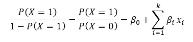
Using elementary math operations we can easily conclude
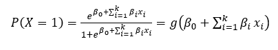
or in a case when n=1:
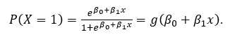
Now we have to estimate coefficients from the given data.
This can be done using a maximum-likelihood estimation (MLE). Many machine learning algorithms use maximum-likelihood estimation as a systematic way of parameter estimation. To give you the idea behind MLE, let us look at an example.
Example: We have a bag that contains three balls, either red (R) or blue (B), but we have no information in addition to this. Thus, the number of blue balls, call it θ, might take values from the set {0, 1, 2, 3}. We can choose four balls at random from the bag with replacement. Let xi, i=1,2,3,4, denotes the color of the ball in its drawing from a bag. After doing our experiment, the following values are observed: x1=B, x2=R, x3=B, x4=B. Thus, we observe three blue balls and one red ball. What is the most probable value for parameter θ?
For each possible value of θ we will find the probability of the observed sample, (x1, x2, x3, x4) = (B, R, B, B).
P(xi=B) =θ/3, P(xi=R) =1-θ/3, i=1, 2, 3, 4.
P(x0=B, x1=R, x2=B, x3=B) = P(x0=B)·P(x1=R)·P(x2=1)·P(x3=1) = θ/3⋅(1-θ/3)⋅θ/3⋅θ/3= (θ/3)^3⋅(1-θ/3)
Note that the joint probability mass function (PMF) depends on θ, so we can write it as P(x1,x2,x3,x4;θ). We obtain the values given in the table for the probability of P(B, R, B, B).
| θ | 0 | 1 | 2 | 3 |
| P | 0 | 2/81 | 8/81 | 0 |
It makes sense that the probability of observed sample for θ=0 and θ=3 is zero, because our sample included both red and blue balls. From the table we can conclude that the probability of the observed data is maximized for θ=2. In other words, the observed data is most likely to occur for θ=2, so we may choose value 2 as our estimate of θ. This is called the maximum likelihood estimate (MLE) of θ. In practice, MLE is usually done using the natural logarithm of the likelihood, known as the log-likelihood function.
Our resulting model will predict a value very close to 1 for the “positive” class and value very close to 0 for the other class. Why is it a good idea to use maximum-likelihood for logistic regression? The search procedure seeks values for the coefficients that minimize the error in the probabilities predicted by the model to those in the data. We will not delve into the math of maximum likelihood (if you want a more detailed math approach, check https://www.geeksforgeeks.org/understanding-logistic-regression/ or An Introduction to Statistical Learning: with Applications in R, pages 130-137). Using training data, we can use a minimization algorithm to find the best values for the coefficients. This is often implemented using gradient descent, BFGS (Broyden–Fletcher–Goldfarb–Shanno algorithm), L-BFGS (BFGS with limited memory), Conjugate Gradient, or some other numerical optimization algorithm.
Example (adapted from https://machinelearningmastery.com/logistic-regression-for-machine-learning/):
We try to predict gender (male or female) based on height (in centimeters). Our learned coefficients for logistic regression are β0 = -100 and β1 = 0.6. If we know the height 165, what is the probability that the person is a man? Using the equation above we can calculate the probability of males given a height of 160cm or, more formally, P(X=’male’ | height=160). We can use spreadsheets or calculators and finally we got: P(X=’male’ | height=160) =0.0179862.
The probability is near zero, so we can say that the person is a female. In this example, we use the probabilities directly, but if we want to use linear regression for the classification we have to introduce the so-called “decision boundary.” For example, we can say: a person is female if g(β_0+β_1 x)<0.5, and the person is male if g(β_0+β_1 x)⩾0.5.
Thanks for reading this article. If you like it, please recommend and share it.