We present a short introduction to one of the most common regression approaches – a linear regression model.
Author: Goran Sukovic, PhD in Mathematics, Faculty of Natural Sciences and Mathematics, University
Linear regression is a special case of the regression analysis – a statistical technique for modeling the relationship between variables. The main idea underlying regression analysis is very simple; how an output feature (or response variable of special interest) depends on one or several other input features, predictors, or explanatory variables. Examples of applied problems and questions in which regression might be useful:
1. predict the happiness, on a scale from 1 to 10, based on the annual income
2. predict forced exhalation volume (FEV), a measure of how much air somebody can forcibly exhale from their lungs, based on the age in years. (“An Exhalent Problem for Teaching Statistics”, The Journal of Statistical Education, 13(2)).
3. determine the sales (in thousands of units) for a product as a function of advertising budgets (in thousands of dollars) for TV, radio, and newspaper media (Gareth James, Daniela Witten, Trevor Hastie, and Robert Tibshirani – “An Introduction to Statistical Learning with Applications in R”, 7th Edition, Springer, 2014)
4. determine the apartment price based on size, location, floor, closeness to bus station/subway station.
5. predict the growth of the plants based on soil quality, humidity, and fertilizer
6. find the height of a child if you know the heights of the parents and nutrition
7. predict the weight, blood pressure, and the cholesterol level based on the eating habits of students (e.g., number of ounces/grams of the red meat, chicken meat, fish, and diary consumed during the one week)
In this article, we review some of the key ideas underlying the linear regression model. Linear regression is one of the simplest parametric approaches for predicting a quantitative response. More formally, a linear regression model with k predictor variables X1 , X2 , …, Xk and a response Y, can be written as y = β0 + β1X1 + β2X2 + · · · βkXk + ε, where the ε is the residual terms of the model. If we use a single predictor variable to predict the value of the output variable, then we talking about simple linear regression. Simple linear regression models are suitable for examples one and two above. The term multiple regression is reserved for models with two or more predictors and one response, such as examples three through six above. Example seven, which represents the models with two or more outputs, is usually called multivariate regression models.
Although there are many “fancier” machine learning and statistical approaches, linear regression is still a very useful and widely used method in medicine, engineering, social sciences, and economy, to mention just a few of the areas. As we see in the following articles, many other methods are developed as generalizations or extensions of the linear regression model.
Even if you are not good at math, it is a good idea to develop some geometric intuition about the linear regression model. Models with one predictor variable and a response variable Y = β0 + β1X1 + ε can be understood as a line in the Cartesian coordinate system. The intercept β0 and the slope β1 are unknown constants, and ε is a random error component. In other words, we can assume that there is approximately a linear relationship between X1 and Y, written as Y ≈ β0 + β1X1, where “≈” can be understood as “is approximately modeled as”. The observations X1 are points in the plane and the line is “fitted” to best approximate the observations. In this case, we interpret variable Y as a continuous dependent variable: X1 is independent variable assumed to be non-random; the random error ε has the following properties: E (ε) = 0 and V (ε) = σ2. To make a prediction using a given formula, we must use a data set to estimate unknown coefficients β0 and β1. Let (x1 , y1), (x2 , y2), . . . , (xn , yn) denotes a data set with n observation pairs. The following figure presents a data set for n = 200 different markets in the Advertising example, where input variable X1 is TV advertising budget and the output variable is product sales in thousands.
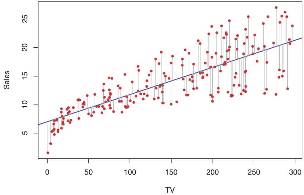
Our goal is to find a line that is the best fit for the data set. In other words, our line should be as close as possible to the given data points. We can use many ways to measure “closeness”. One of the most common methods measuring “closeness” is to minimize the least-squares error. Soon we will discuss alternative methods.
Let f(xi)= β0+ β1xi be the prediction for output Y based on the ith value of X. Then, for each i, calculate the difference between the observed response value and the value predicted by our model: ei = yi − f(xi). This value is known as ith residual. The residual sum of squares (RSS) is defined as e12+e22+…+en2, or equivalently as (y1-f(x1))2+(y2-f(x2))2+…+(yn-f(xn))2. Using common methods to minimize real-valued functions of two variables, we can easily find a closed formula for unknown coefficients.
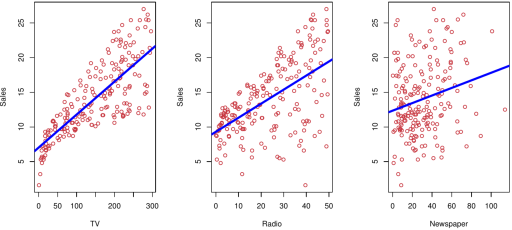
Example: Advertising data set from example three above, from the book Gareth James, Daniela Witten, Trevor Hastie and Robert Tibshirani – “An Introduction to Statistical Learning with Applications in R”, 7th Edition, Springer, 2014. The following figure presents three different simple regression models, based respectively on variables TV, radio and newspaper:
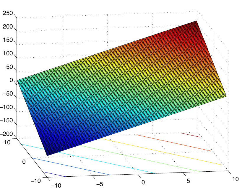
Multiple regression models with two predictor variables X1 and X2 and a response variable y = β0 + β1X1 + β2X2 + ε can be understood as a plane in space. Similarly, to the case of the simple linear regression, the observations are points in space and the plane is “fitted” to best approximate the observations.
Example: From the lecture notes M. Bremer, Math 261 A, 2012. For model y = 50β0 + 10β1X1 + 7β2X2, plane looks like this:
Let f(xi)= β0+ β1x1+ β2x2 + … + βnxn be the prediction for output Y based on the ith value of X. The formula for the residual sum of squares (RSS) for multiple regression is the same as in a case for simple linear regression. As before, we could use some calculus to determine values of the model parameters: find derivatives with respect to β0 , . . . , βk , set them equal to zero, and derive the equations that our parameter would have to fulfill.
We gave a short introduction to one of the most common regression approaches – linear regression model. The model belongs to parametric supervised machine learning algorithms. Soon we will discuss how to assess the accuracy of the coefficient estimate.
Thanks for reading this article. If you like it, please recommend and share it.